Chapter6 シュレディンガー方程式
6.1 1次元自由粒子のシュレディンガー方程式
電子の波動,つまりド・ブロイ波の正体が何かはわかっていません.しかし,波動である限り,波動についての一般量
![]() が存在するはずです.(古典論の場合,
が存在するはずです.(古典論の場合,
![]() の例としては,水波の場合の変位であったり,音波の場合の密度であったり,電磁波の場合の電場や磁場であったりします.)このド・ブロイ波の
の例としては,水波の場合の変位であったり,音波の場合の密度であったり,電磁波の場合の電場や磁場であったりします.)このド・ブロイ波の
![]() の満たす方程式を導出してみましょう.簡単のため,
の満たす方程式を導出してみましょう.簡単のため,![]() 方向のみの1次元の場合を考えます.
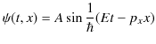
方向のみの1次元の場合を考えます.![]() の関数形は種々あるでしょうが,次の正弦波の場合を取り上げます.
の関数形は種々あるでしょうが,次の正弦波の場合を取り上げます.
![]() は振幅,
は振幅,![]() は角振動数,
は角振動数,![]() は波数です.この最も簡単な波動である正弦波は,最も簡単な粒子の運動状態である自由粒子に対応することができると仮定します.(この仮定が正しいことは,後で,"束縛状態(例: 自由粒子と井戸型ポテンシャル)" のChapterで確認されます.)ここで,アインシュタイン-ド・ブロイの関係式,
は波数です.この最も簡単な波動である正弦波は,最も簡単な粒子の運動状態である自由粒子に対応することができると仮定します.(この仮定が正しいことは,後で,"束縛状態(例: 自由粒子と井戸型ポテンシャル)" のChapterで確認されます.)ここで,アインシュタイン-ド・ブロイの関係式,
より,
となります.この ![]() を1次元波動方程式,
を1次元波動方程式,
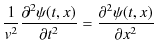
に代入してみましょう.![]() を
を ![]() で微分していくと,
で微分していくと,
 |
||
 |
となります.![]() を
を ![]() で微分していくと,
で微分していくと,
 |
||
 |
となります.したがって,これらを1次元波動方程式に代入して,
 |
||
が導かれます.しかし,この式は古典論での自由粒子に対するエネルギーと運動量の関係である,

には一致しません.
そこで,![]() に対する波動方程式は,波動一般に成立する上記のものではなく,
に対する波動方程式は,波動一般に成立する上記のものではなく,
のような,形をした方程式になると思われます.この形の方程式からは,![]() については1次,
については1次,![]() については2次の関係が出てきます.
については2次の関係が出てきます.![]() はある定数であり,今から決定するべきものです.このとき,もはや,
はある定数であり,今から決定するべきものです.このとき,もはや,![]() は最初の,
は最初の,
の形では,方程式を満たすことができません.つまり,
|
||
|
という2つの式は,任意の位相(正弦や余弦の角度部分)について,イコールでは結ばれません.そこで,
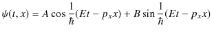
と置き直し,![]() と
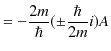
と ![]() を求めることにします.まず,
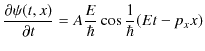
を求めることにします.まず,![]() を
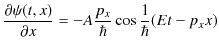
を ![]() について偏微分します.
について偏微分します.
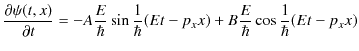
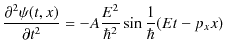
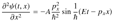
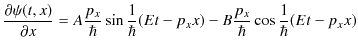
次に,![]() を
を ![]() で2回偏微分します.
で2回偏微分します.
 |
||
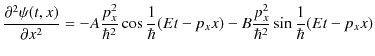 |
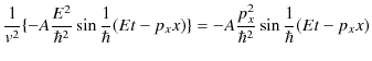
ここで,(6.1)式より,

となりますが,任意の位相について,イコールが成立するとします.このとき,正弦と余弦の係数をそれぞれ比較して,
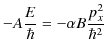 |
||
 |
となり,故に,
 |
||
 |
の関係が成立します.ここで,自由粒子の場合の関係,
を使うと,
 |
||
 |
となります.したがって,
 |
||
 |
||
 |
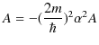
と ![]() が求められます.さらに,
が求められます.さらに,![]() を求めると,
を求めると,
 |
||
となります.(複号同順.)この ![]() を元の
を元の ![]() の式に代入して計算します.
の式に代入して計算します.
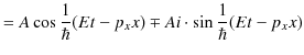 |
||
 |
||
 |
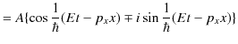
この場合,複号はどちらをとっても良いです.また,![]() は振幅であると考えられます.この
は振幅であると考えられます.この ![]() は確かに正弦波の形をしています.しかし,複素数の波動になっています.古典論では,微分方程式の解で複素数が出てきた場合は,ことごとく虚数部を捨て,実数部のみを現実の解とすることが常套手段です.しかし,波動力学では,複素数そのものが実在であると考えるのです.そして,この複素数の
は確かに正弦波の形をしています.しかし,複素数の波動になっています.古典論では,微分方程式の解で複素数が出てきた場合は,ことごとく虚数部を捨て,実数部のみを現実の解とすることが常套手段です.しかし,波動力学では,複素数そのものが実在であると考えるのです.そして,この複素数の ![]() をシュレディンガーは波動関数と名付けました.波動関数はド・ブロイ波から生まれた概念です.概念の発展の繋がりを示しておきます.
をシュレディンガーは波動関数と名付けました.波動関数はド・ブロイ波から生まれた概念です.概念の発展の繋がりを示しておきます.
"ド・ブロイ波→波動関数 ![]() (複素数)"
(複素数)"
一方,(6.1)式に ![]() を代入します.
を代入します.
 |
||
 |
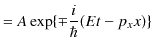
となります.複号は通常の表記に従って,上の符号を採ることにします.つまり,
とします.また,複号で上の符号を選んだので,上記の波動関数は,
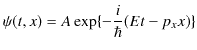
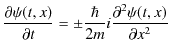
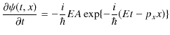
となります.この波動関数を,(6.2)式に代入して,自由粒子に対するエネルギーと運動量の関係式,
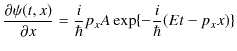
が成立していることを確認しておきましょう.![]() を
を ![]() で1回偏微分して,
で1回偏微分して,
となります.![]() を
を ![]() で2回偏微分して,
で2回偏微分して,
 |
||
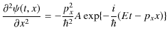 |
となります.これらを(6.2)式に代入して計算します.
![$\displaystyle i\hbar[-\dfrac{i}{\hbar}EA\exp\{-\dfrac{i}{\hbar}(Et-p_{x}x)\}]=-...
...ar^{2}}{2m}[-\dfrac{p_{x}^{2}}{\hbar^{2}}A\exp\{-\dfrac{i}{\hbar}(Et-p_{x}x)\}]$](ja_Chapter6_SchrodingerEquation_images/img61.png)
よって,
となり,
と確かに導かれます.つまり,自由粒子のエネルギーと運動量の関係式を満たす波動方程式(6.2)式が求められたことになり,当初の目的が達成されました.(6.2)式を自由粒子の1次元シュレディンガー方程式といいます.
6.2 量子化
(6.3)式を見ると,波動関数に古典論の自由粒子に対するエネルギーと運動量の関係式がかけられていることがわかります.この式をヒントにして,古典論から波動力学の方程式を導くことを考えましょう.(6.3)式から(6.2)式を導く方法として,
 |
||
 |
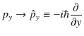
の置き換えをすればよいことがわかります.(![]() の上にある記号ハットは,それが演算子であることを示します.)書き直すと,運動量については,
の上にある記号ハットは,それが演算子であることを示します.)書き直すと,運動量については,
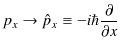
とすればよいです.この古典的物理量から演算子への置き換えを量子化といいます.ここで,自由粒子に対する,古典論から波動力学へ移行する手続きをまとめておきましょう.
- 古典論での物理量の間の関係式を求めます.
- 量子化により古典的物理量を演算子に置き換え,演算子の間の関係式を導きます.
- 演算子の関係式を波動関数に左からかけます.(演算子をかけることを作用するといいます.)
自由粒子の場合を考えて,以上の手続きを導入しましたが,この手続きは一般的に採用される方法です.量子化を手掛かりにして,一般の場合のシュレディンガー方程式を求めていきましょう.
6.3 一般的なシュレディンガー方程式
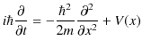
(6.2)式を力がはたらいている場合,つまり,ポテンシャル ![]() がある場合について拡張しましょう.古典論では,
がある場合について拡張しましょう.古典論では,
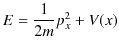
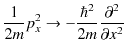
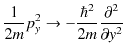
の関係式があります.ここで,量子化,
|
||
|
を行い,演算子に置き換えます.このとき,
となりました.また,ポテンシャル ![]() は座標
は座標 ![]() の関数ですが,座標
の関数ですが,座標 ![]() の量子化は,
の量子化は,
であることが知られています.つまり,座標 ![]() については波動力学でも,古典論と同様に
については波動力学でも,古典論と同様に ![]() のままです.したがって,ポテンシャルは量子化されても
のままです.したがって,ポテンシャルは量子化されても ![]() のままです.すなわち,量子化後の演算子の間の関係式は,
のままです.すなわち,量子化後の演算子の間の関係式は,
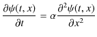
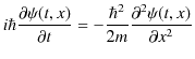
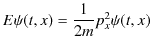
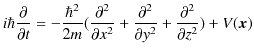
となります.この式の両辺を波動関数 ![]() に作用させて,
に作用させて,
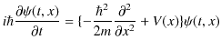
が成立します.この式を1次元シュレディンガー方程式といいます.
さらに,3次元に拡張します.3次元の場合,エネルギーについての古典的関係式は,
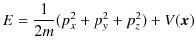
です.ここで,量子化,
|
||
|
||
 |
||
 |
を行い,演算子に置き換えます.このとき,
|
||
 |
||
 |
となります.ポテンシャルは波動力学でも変わらず ![]() のままです.このとき,演算子の間の関係式は,
のままです.このとき,演算子の間の関係式は,
です.この式の両辺を波動関数
![]() に左から作用させて,
に左から作用させて,
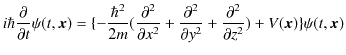
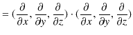
が成立します.ここで,よく使用される記号であるナブラ
![]() を定義します.
を定義します.
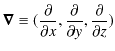
![]() と
と
![]() で内積をとります.
で内積をとります.
 |
||
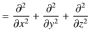 |
となりますので,上記の方程式は次のように表されます.
この方程式こそが波動力学の基礎方程式であるシュレディンガー方程式です.ここで,以上の議論はシュレディンガー方程式の証明にはなっていないことに注意しましょう.この方程式が正しいことを実証する方法は,様々な場合について,この微分方程式を解き,その結果が実験に一致することを確認しなければなりません.長い年月の検証に耐え,シュレディンガー方程式は,ニュートン力学において運動方程式が果たした役割を,波動力学において担い続けているのです.
6.4 ハミルトニアン
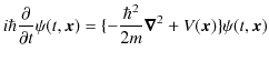
3次元におけるエネルギーについての古典的関係式,
の右辺は,解析力学ではハミルトニアンそのものです.
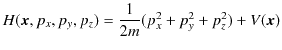
ハミルトニアンは対象にしている物理系を記述する古典的物理量です.このハミルトニアンを量子化して,波動力学での系を記述する物理量として使用することができます.一般に,波動力学はハミルトニアン形式で記述されるのです.ハミルトニアンを量子化すると,
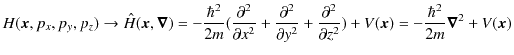
となります.このとき,シュレディンガー方程式は,
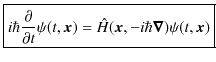
と書き直されます.
6.5 時間に依存しないシュレディンガー方程式
波動関数の物理的な意味を考えるのは,次のChapterで行いますが,波動に関する何らかの量であることは間違いありません.波動一般について,時間的に進行しない定常波という状態が存在しました.波動関数が定常波を形成して,時間的に進行しない場合,シュレディンガー方程式がどのようになるのかを考えてみましょう.波動関数
![]() が次式のように,時間だけの関数
が次式のように,時間だけの関数 ![]() と空間だけの関数
と空間だけの関数
![]() との積で表される場合を取り扱います.
との積で表される場合を取り扱います.
このとき,関数
![]() は時間に依存しません.この式をシュレディンガー方程式(6.4)式に代入します.
は時間に依存しません.この式をシュレディンガー方程式(6.4)式に代入します.
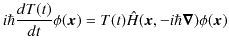
両辺を
![]() で割ると,
で割ると,
となります.この等式において,左辺は ![]() だけの関数であり,右辺は
だけの関数であり,右辺は ![]() だけの関数です.これらが恒等的に等しくなるためには定数にならなければなりません.この定数を
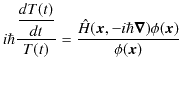
だけの関数です.これらが恒等的に等しくなるためには定数にならなければなりません.この定数を ![]() とおきます.このとき,
とおきます.このとき,
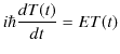
と,
の2式が得られます.(6.5)式の左辺は
![]() にハミルトニアンがかかっています.したがって,右辺の
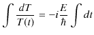
にハミルトニアンがかかっています.したがって,右辺の ![]() はエネルギーと考えられます.また,第1式を解くと,
はエネルギーと考えられます.また,第1式を解くと,
 |
||
 |
||
 |
||
 |
||
 |
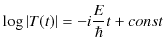
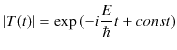
となります.ただし,最後の式は ![]() を置き直しました.故に,
を置き直しました.故に,
となりますが,さらに,![]() を
を ![]() と置き直して,
と置き直して,
となります.ここで,![]() はエネルギーであったので,アインシュタイン-ド・ブロイの関係式,
はエネルギーであったので,アインシュタイン-ド・ブロイの関係式,
より,
となります.したがって,
![]() は定常波のそれぞれの座標での振幅を表し,
は定常波のそれぞれの座標での振幅を表し,![]() は定常波の各座標における振動の時間的変化を表していると考えられます.前述した(6.4)式を時間に依存するシュレディンガー方程式といいます.それに対して,(6.5)式を時間に依存しないシュレディンガー方程式といいます.また,
は定常波の各座標における振動の時間的変化を表していると考えられます.前述した(6.4)式を時間に依存するシュレディンガー方程式といいます.それに対して,(6.5)式を時間に依存しないシュレディンガー方程式といいます.また,
![]() を時間に依存する波動関数,
を時間に依存する波動関数,
![]() を時間に依存しない波動関数といいます.ここで,
を時間に依存しない波動関数といいます.ここで,![]() の式を
の式を
![]() に代入して,
に代入して,
![]() と
と
![]() の間に,
の間に,
の関係があることがわかります.